FLASH FILL: Excel 2013 has an awesome feature called Flash Fill. How does Flash Fill work? It gives you the ability to take a part of the data entered in a column of a worksheet table, type part of it into the next column over, and fill a series.
Excel detects patterns in your initial data entry! The application then figures out the data you want to copy and even offers a few choices to match exactly what you want. Fill a series without a formula! Instead of manually entering your data or copying and pasting, let Excel do the work. Here’s how...
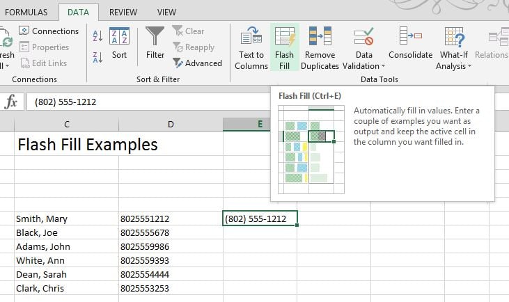
1. Column A has the last name, a comma and a first name. As long as you begin typing in a column that touches the data, Flash Fill will work! Type Mary Smith, for example. Press Enter. Start typing in Joe Black and you’ll see Excel work its magic! You’ll see grey suggestions and if you’re happy, press Enter and the column will fill without the use of a formula.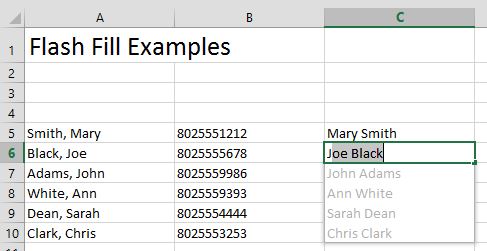
2. The same thing can be done with phone numbers, for example. If you want to quickly change the format of simple data entries, use the same method as step one. Type in the phone number format that you would like to use and Flash Fill will notice the pattern. You’ll also get options to Undo Flash Fill, Accept suggestions and Select all changed cells. 
3. Another way to apply Flash Fill is to type in the format that you would like and click on the Data tab. In the Data Tools group, click on Flash Fill.
4. Don’t be afraid to try different combinations to make your life easier. If a company uses the same naming convention for email addresses, try that. You could also pull names out of an email address using Flash Fill. This is a quick and easy way to save some time without writing formulas and using functions and end up with constant values. This feature is available in Excel 2013. 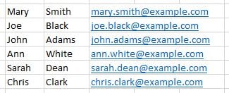
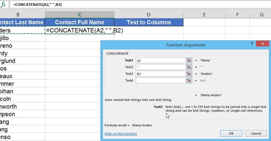
CONCATENTATE: The CONCATENATE function allows you to join up to 255 text strings into one text string. This is best used in Excel 2010. It can be text, numbers, cell references, or a combination. For example, your worksheet may contain a person's first name in cell A4 and their last name in cell B4. How can you combine the two values in another cell? Try this:
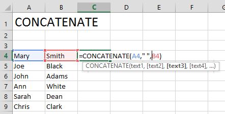
1. In this example, type =CONCATENATE(A4," ",B4) in the destination cell. CONCATENATE is the function, A4 is the first argument or string and then a comma.
2. The second argument in this example (" ") is a space character. With this function, each argument must be a string. If you leave out the space character, there will not be a space between the first name and the last name.
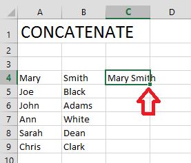
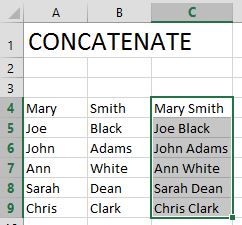
3. Then just copy the formula down either by dragging or double clicking on the bottom right of the cell. Remember, this is a formula so you will need to copy and paste as constant values.
Another option is to click on the ![]() button to open the Function Arguments dialog box. This will walk you through the steps for each string and even show you the results before you click OK to accept it.
button to open the Function Arguments dialog box. This will walk you through the steps for each string and even show you the results before you click OK to accept it.
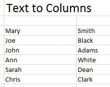
TEXT TO COLUMNS: Use the Convert Text to Columns Wizard to separate simple cell content, such as first names and last names into different columns.
Depending on your data, you can split the cell content based on a delimiter such as a space, a comma or based on a specific column break location within your data.
1. Select the range of data that you want to convert.
2. On the Data tab, in the Data Tools group, click Text to Columns.
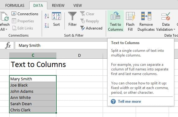
3. In Step 1 of the Convert Text to Columns Wizard, click Delimited (which is a separator) and then click Next.
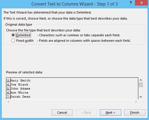
4. In Step 2, select the Space check box and clear the other check boxes under Delimiters.
5. The Data preview box shows the first and last names in two separate columns.
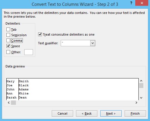
6. Click Next.
7. Click a column in the Data preview box and click General under Column data format.
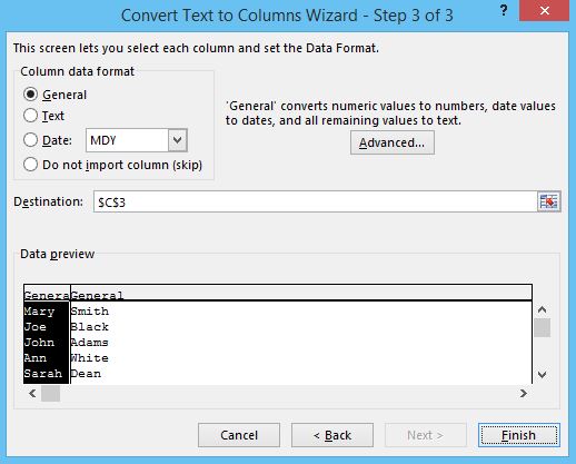
8. If you want to insert the separated content into the columns next to the full name, click the icon to the right of the Destination box and select the cell next to the first name in the list. The split data will replace the original data if you don't specify a new destination for the new columns.

