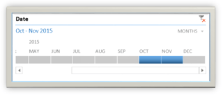
 Have you ever used Slicers in Excel? Slicers make it easy for users to filter tables, PivotTables, and PivotCharts. Timeline is a new feature to Excel 2013 that is similar to Slicers except it allows users to filter dates interactively. This is a must for anyone reporting using dates. Dates can be easily filtered by days, months, quarters, and years. Follow the steps below to learn how to insert and use a Timeline in your PivotTable in Excel.
1. Click in your data that contains dates, and create a PivotTable (Insert tab / PivotTable).
2. While still in the PivotTable, click on the Insert tab / Filters group / Timeline.

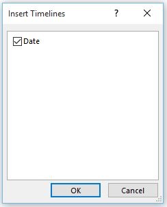
3. In the Insert Timelines Dialog box check the appropriate box and click OK.
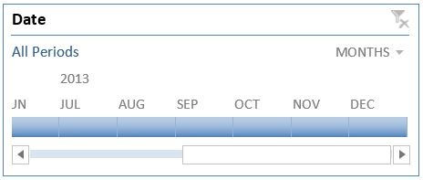
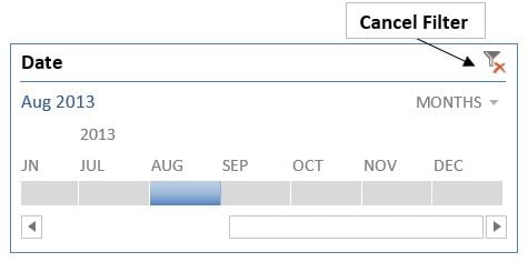
4. A Timeline scale will appear. It can be moved and resized if necessary.
5. To filter your PivotTable data, either click on the specific date time or choose from one of the many filtering options located under the drop list.
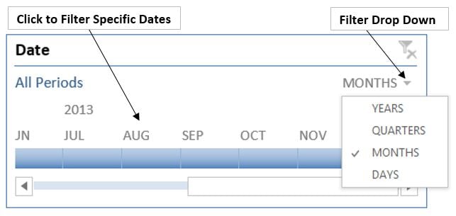
6. Click on the Cancel Filter button to view all results.
If you enjoyed this tip, we invite you to check out our FREE video on 10 AHA! Moments in Microsoft Excel.


